
2. Unconfined Aquifer Test - Vennebulten#
Import packages#
import matplotlib.pyplot as plt
import numpy as np
import pandas as pd

import timflow.transient as tft

plt.rcParams["figure.figsize"] = (5, 3)  # default figure size
Introduction and Conceptual Model#
In aquifer tests in unconfined aquifers, there is also the vertical component to flow to the well. The drawdown data shows the delayed water table response, a distinguishable S-shape in the log-log plot. In the early times of the drawdown, the drawdown behaves as a confined aquifer: when the aquifer releases the elastic storage. However, as pumping continues, the water table storage begins to be released, generating further drawdown and the S-shape.
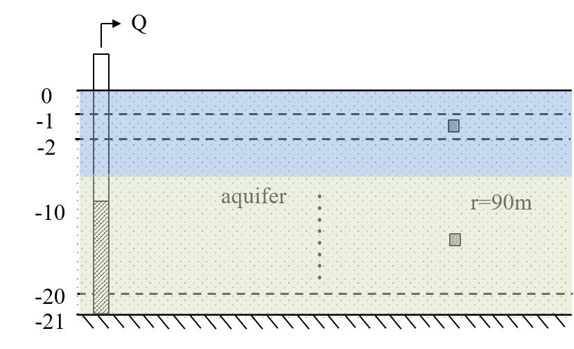
This test conducted in Vennebulten, the Netherlands, is reported in Kruseman et al. (1970). The cross-section consists of a first layer up to 6 m depth of very fine and loamy sands, followed by coarse sands until 21 m deep.
The screen of the pumping well is placed between 10 and 21 meters depth, and pumping has taken place for 25 hours at a rate of 873 m3/d. The available drawdown data comes from two piezometers, a shallow one, screened at 3 m depth, and a deeper one, screened in the depths between 12 to 19 m. Both wells are located 90 m from the pumping well.
Load data#
data1 = np.loadtxt("data/venne_shallow.txt", skiprows=1)
ts = data1[:, 0] / 60 / 24  # convert min to days
hs = data1[:, 1]

data2 = np.loadtxt("data/venne_deep.txt", skiprows=1)
td = data2[:, 0] / 60 / 24  # convert min to days
hd = data2[:, 1]
Parameters and model#
b = -21  # aquifer thickness, m
r = 90  # distance from observation wells to pumping well, m
Q = 873  # constant discharge, m^3/d
k = 12 * [0.5] + 15 * [150]
z = np.hstack((np.arange(0, -6, -0.5), np.arange(-6, -21.1, -1)))
Ss = [0.2] + 26 * [1e-4]
kzoverkh = 0.1
ml = tft.Model3D(
    kaq=k,
    z=z,
    Saq=Ss,
    kzoverkh=kzoverkh,
    topboundary="phreatic",
    tmin=1e-4,
    tmax=1.1,
)
w = tft.Well(ml, xw=0, yw=0, rw=0.1, tsandQ=[(0, Q)], layers=range(10, 21))
wobs = tft.Well(ml, xw=90, yw=0, rw=0.1, tsandQ=[(0, 0)], layers=range(18, 27))
ml.solve()
self.neq  20
solution complete
Estimate aquifer parameters#
cal = tft.Calibrate(ml)

cal.set_parameter(
    name="Saq", initial=1e-4, layers=list(range(1, 12)), pmin=1e-6, pmax=1e-2
)
cal.set_parameter(name="kaq", initial=150, layers=list(range(0, 12)), pmin=0.05, pmax=1)

cal.set_parameter(
    name="Saq", initial=1e-4, layers=list(range(12, 27)), pmin=1e-6, pmax=1e-2
)
cal.set_parameter(name="kaq", initial=150, layers=list(range(12, 27)), pmin=100, pmax=200)

cal.series(name="shallow_obs", x=r, y=0, t=ts, h=hs, layer=5)
cal.seriesinwell(name="wobs", element=wobs, t=td, h=hd)

cal.fit(report=True)
...............................................................................
Fit succeeded.
[[Fit Statistics]]
    # fitting method   = leastsq
    # function evals   = 76
    # data points      = 48
    # variables        = 4
    chi-square         = 0.00319397
    reduced chi-square = 7.2590e-05
    Akaike info crit   = -453.649150
    Bayesian info crit = -446.164346
[[Variables]]
    Saq_1_11:   1.3997e-04 (init = 0.0001)
    kaq_0_11:   0.08061669 (init = 1)
    Saq_12_26:  2.9428e-05 (init = 0.0001)
    kaq_12_26:  121.610702 (init = 150)
......
.
.......
.
.......
.
......
.
.......
.
......
.
.......
.
.......
.
.......
.
.......
.
.
Fit succeeded.
[[Fit Statistics]]
    # fitting method   = leastsq
    # function evals   = 76
    # data points      = 48
    # variables        = 4
    chi-square         = 0.00319397
    reduced chi-square = 7.2590e-05
    Akaike info crit   = -453.649150
    Bayesian info crit = -446.164346
[[Variables]]
    Saq_1_11:   1.3997e-04 (init = 0.0001)
    kaq_0_11:   0.08061669 (init = 1)
    Saq_12_26:  2.9428e-05 (init = 0.0001)
    kaq_12_26:  121.610702 (init = 150)
display(cal.parameters.loc[:, ["optimal"]])
print(f"RMSE: {cal.rmse():.3f} m")
| optimal | |
|---|---|
| Saq_1_11 | 0.000140 |
| kaq_0_11 | 0.080617 |
| Saq_12_26 | 0.000029 |
| kaq_12_26 | 121.610702 |
RMSE: 0.008 m
hs_1 = ml.head(r, 0, ts, layers=3)
hd_1 = wobs.headinside(td)

plt.semilogx(ts, hs, ".", label="shallow obs")
plt.semilogx(ts, hs_1[0], label="shallow ttim")
plt.semilogx(td, hd, ".", label="deep obs")
plt.semilogx(td, hd_1[0], "--", label="deep ttim")
plt.xlabel("time [d]")
plt.ylabel("head change [m]")
plt.title("Timflow Unconfined Model Results - Shallow Piezometer")
plt.legend()
plt.grid()
Comparison of results#
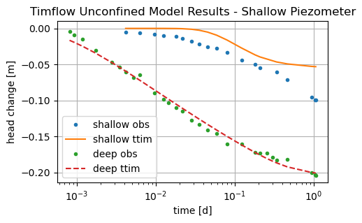
The performance of timflow is compared with a model performed with MLU (Hemker & Post, 2014). The schematization of the MLU model differs considerably. The model consists of three layers: a very thin fine-grained upper aquifer layer with horizontal flow and two deeper sublayers with a thickness of 1 and 10 meters. In total, four parameters were estimated (Ss0, c2, Ss2, k2), while fixed values were chosen for the remaining ones.
The RMSE of MLU is smaller than that of timflow, but MLU uses more layers with fixed parameters.
| Ss0 [1/m] | k0 [m/d] | c1 [d] | Ss1 [1/m] | k1 [m/d] | c2 [d] | Ss2 [1/m] | k2 [m/d] | RMSE [m] | |
|---|---|---|---|---|---|---|---|---|---|
| timflow | 1.40e-04 | 0.08 | - | 2.94e-05 | 121.61 | - | - | - | 0.0082 |
| MLU | 3.80e-01 | 1.00 | 100 | 1.00e-06 | 50.00 | 209 | 5.58e-03 | 165.90 | 0.0005 |
References#
Hemker, K. en Post V. (2014) MLU for Windows: well flow modeling in multilayer aquifer systems; MLU User’s guide
Kruseman, G.P., De Ridder, N.A., Verweij, J.M., 1970. Analysis and evaluationof pumping test data. volume 11. International institute for land reclamation and improvement The Netherlands.
Neuman, S.P., Witherspoon, P.A., 1969. Applicability of current theories of flow in leaky aquifers. Water Resources Research 5, 817–829.