Connected Wells#
WellString elements can be used to model a series of connected wells. There are several types of WellString:
WellString: connected wells with equal head inside the wells and a user-specified total discharge
This notebook shows how to model the WellString element with two wells
and compares the results to models with two individual wells, which should give the same answer for this simple case with only two wells pumping in an infinite aquifer. Examples are shown for both
elements in single- and multi-layer models.
import matplotlib.pyplot as plt
import numpy as np

import timflow
import timflow.transient as tft
timflow.show_versions()
timflow version    : 0.4.1

Python version     : 3.13.14
Numpy version      : 2.4.6
Numba version      : 0.66.0
Scipy version      : 1.18.0
Pandas version     : 3.0.3
Matplotlib version : 3.11.0
LmFit version      : 1.3.4
WellString#
A series of wells that have equal head (pressure) inside the well and pump with a total specified discharge.
Single-layer model#
# model parameters
kh = 10  # m/day
Ss = 1e-4  # 1/m

ctop = 1000.0  # resistance top leaky layer in days

ztop = 0.0  # surface elevation
zbot = -20.0  # bottom elevation of the model

z = [1.0, ztop, zbot]
kaq = np.array([kh])
Ss = np.array([Ss])
c = np.array([ctop])

Qtot = 100
Reference model with 2 wells with equal discharge of Qtot / 2
mlref = tft.ModelMaq(kaq=kaq, Saq=Ss, c=c, z=z, topboundary="semi", tmin=0.1, tmax=10)
w1 = tft.Well(mlref, 0, -10, tsandQ=(0, Qtot / 2), rw=0.1)
w2 = tft.Well(mlref, 0, 10, tsandQ=(0, Qtot / 2), rw=0.1)
mlref.solve()
self.neq  2
solution complete
Model with a WellString that has total discharge equal to the sum of the two discharge-specified wells. This should give the same solution.
ml = tft.ModelMaq(kaq=kaq, Saq=Ss, c=c, z=z, topboundary="semi", tmin=0.1, tmax=10)
ws = tft.WellString(ml, xy=[(0, -10), (0, 10)], tsandQ=(0, Qtot), rw=0.1)
ml.solve()
self.neq  2
solution complete
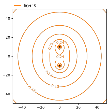
Contour the heads of the first reference model and the WellString model.
time = 0.2
levels = 10
ax = mlref.plots.topview(win=(-50, 50, -50, 50))
mlref.plots.contour(
    win=(-50, 50, -50, 50),
    ngr=51,
    t=time,
    levels=levels,
    decimals=2,
    layers=[0],
    ax=ax,
)
ml.plots.contour(
    win=(-50, 50, -50, 50),
    ngr=51,
    t=time,
    levels=levels,
    decimals=2,
    layers=[0],
    color="C1",
    ax=ax,
);
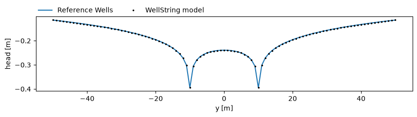
Compare heads along y between the two models.
y = np.linspace(-50, 50, 101)
x = np.zeros_like(y)
href = mlref.headalongline(x, y, t=time)
h0 = ml.headalongline(x, y, t=time)

plt.figure(figsize=(10, 2))
plt.plot(y, href[0, 0], label="Reference Wells")
plt.plot(y, h0[0, 0], "k.", ms=3, label="WellString model")
plt.xlabel("y [m]")
plt.ylabel("head [m]")
plt.legend(loc=(0, 1), frameon=False, ncol=3);
Check computed discharges
# 2 discharge wells, Q specified not computed
w1.discharge(time), w2.discharge(time)
(array([[49.99999901]]), array([[49.99999901]]))
# WellString
ws.discharge_per_well(time)
array([[[49.99999921],
        [49.99999922]]])
Compare heads inside the wells
# 2 discharge wells
w1.headinside(time), w2.headinside(time)
(array([[-0.39493396]]), array([[-0.39493396]]))
# WellString
ws.headinside(time), ws.wlist[0].headinside(time), ws.wlist[1].headinside(time)
(array([-0.39493396]), array([[-0.39493396]]), array([[-0.39493396]]))
Multilayer model#
The following example compares the WellString element to the reference models with 2 individual Wells in an aquifersystem consisting of 3 layers. All wells are screened in the bottom two aquifers.
# model parameters
kh = [5, 10, 20]  # m/day
Ss = 1e-4  # 1/m

c = [1000.0, 100.0, 10.0]  # resistance leaky layers in days

ztop = 0.0  # surface elevation
zbot = -50.0  # bottom elevation of the model

z = [1.0, ztop, -10, -15, -25, -26, zbot]
kaq = np.array(kh)
c = np.array(c)
Reference model with discharge wells
mlref = tft.ModelMaq(kaq=kaq, Saq=Ss, c=c, z=z, topboundary="semi", tmin=0.1, tmax=10)
w1 = tft.Well(mlref, 0, -10, tsandQ=[(0, Qtot / 2)], rw=0.1, layers=[1, 2])
w2 = tft.Well(mlref, 0, 10, tsandQ=[(0, Qtot / 2)], rw=0.1, layers=[1, 2])
mlref.solve()
self.neq  4
solution complete
Model with WellString
ml = tft.ModelMaq(kaq=kaq, Saq=Ss, c=c, z=z, topboundary="semi", tmin=0.1, tmax=10)
ws = tft.WellString(ml, xy=[(0, -10), (0, 10)], tsandQ=[(0, Qtot)], rw=0.1, layers=[1, 2])
ml.solve()
self.neq  4
solution complete
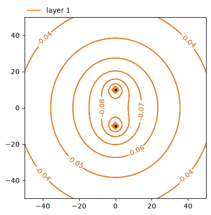
Compare head contours
time = 0.2
ilay = 1
levels = 10
ax = mlref.plots.topview(win=(-50, 50, -50, 50))
mlref.plots.contour(
    win=(-50, 50, -50, 50),
    ngr=51,
    t=time,
    levels=levels,
    decimals=2,
    layers=[ilay],
    ax=ax,
)
ml.plots.contour(
    win=(-50, 50, -50, 50),
    ngr=51,
    t=time,
    levels=levels,
    decimals=2,
    layers=[ilay],
    color="C1",
    ax=ax,
);
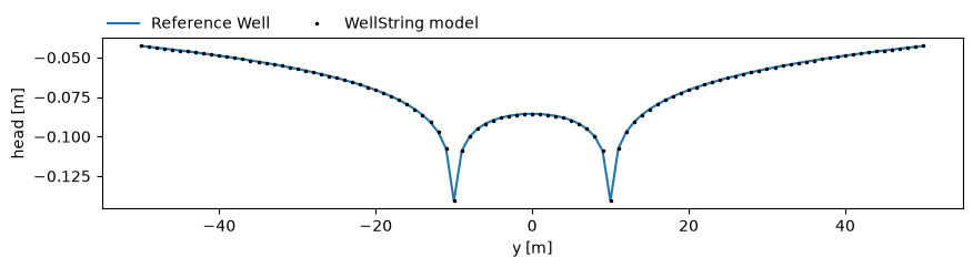
Compare drawdowns along \(y\) in layer 1
y = np.linspace(-50, 50, 101)
x = np.zeros_like(y)
href = mlref.headalongline(x, y, t=time)
h = ml.headalongline(x, y, t=time)

ilay = 1
plt.figure(figsize=(10, 2))
plt.plot(y, href[ilay, 0], label="Reference Well")
plt.plot(y, h[ilay, 0], "k.", ms=3, label="WellString model")
plt.xlabel("y [m]")
plt.ylabel("head [m]")
plt.legend(loc=(0, 1), frameon=False, ncol=3);
Compare discharges
# 2 discharge wells, total Q specified
w1.discharge(time), w2.discharge(time)
(array([[ 8.84723119],
        [41.152768  ]]),
 array([[ 8.84723014],
        [41.15276815]]))
# WellString, transposed to compare to above
ws.discharge_per_well(time).T
array([[[ 0.        ,  8.84723191, 41.1527688 ],
        [ 0.        ,  8.84723094, 41.15276825]]])
Compare heads
# 2 discharge wells
w1.headinside(time), w2.headinside(time)
(array([[-0.14080233],
        [-0.14080233]]),
 array([[-0.14080232],
        [-0.14080233]]))
ws.headinside(time), ws.wlist[0].headinside(time), ws.wlist[1].headinside(time)
(array([-0.14080234]),
 array([[-0.14080234],
        [-0.14080233]]),
 array([[-0.14080233],
        [-0.14080233]]))
Multi-layer with skin effect#
mlref = tft.ModelMaq(kaq=kaq, Saq=Ss, c=c, z=z, topboundary="semi", tmin=0.1, tmax=10)
w1 = tft.Well(mlref, 0, -10, tsandQ=[(0, Qtot / 2)], rw=0.1, res=0.1, layers=[1, 2])
w2 = tft.Well(mlref, 0, 10, tsandQ=[(0, Qtot / 2)], rw=0.1, res=0.1, layers=[1, 2])
mlref.solve()
self.neq  4
solution complete
ml = tft.ModelMaq(kaq=kaq, Saq=Ss, c=c, z=z, topboundary="semi", tmin=0.1, tmax=10)
ws = tft.WellString(
    ml, xy=[(0, -10), (0, 10)], tsandQ=[(0, Qtot)], rw=0.1, res=0.1, layers=[1, 2]
)
ml.solve()
self.neq  4
solution complete
Compare discharges
# 2 discharge wells, total Q specified
w1.discharge(time), w2.discharge(time)
(array([[12.63712098],
        [37.36287809]]),
 array([[12.63712047],
        [37.36287894]]))
# WellString, transposed to compare to above
ws.discharge_per_well(time).T
array([[[ 0.        , 12.6371208 , 37.36287837],
        [ 0.        , 12.63712063, 37.36287905]]])
Compare heads
# 2 discharge wells
w1.headinside(time), w2.headinside(time)
(array([[-0.3803186 ],
        [-0.38031859]]),
 array([[-0.38031859],
        [-0.38031859]]))
ws.headinside(time), ws.wlist[0].headinside(time), ws.wlist[1].headinside(time)
(array([-0.3803186]),
 array([[-0.3803186 ],
        [-0.38031859]]),
 array([[-0.38031859],
        [-0.38031859]]))
Well string with 3 wells#
In general, the discharge of each individual well in a well string will differ depending on the setting. Here is a simple example of a string with three wells. The solution will show that the discharge of the cell in the middle is less than the other two cells, but the total discharge of all three wells is the specified Qtot and the heads in the three wells are equal at all times. The aquifer is changed to confined.
ml = tft.ModelMaq(
    kaq=kaq, Saq=Ss, c=[800, 400], z=z[1:], topboundary="conf", tmin=0.1, tmax=10
)
ws = tft.WellString(
    ml, xy=[(0, -10), (0, 0), (0, 10)], tsandQ=[(0, Qtot)], rw=0.1, res=0.1, layers=[1, 2]
)
ml.solve()
self.neq  6
solution complete
Discharges
time = 0.2
# WellString, transposed to compare to above
ws.discharge_per_well(time).T
array([[[ 0.        ,  8.04179567, 25.65851477],
        [ 0.        ,  7.66308043, 24.93629571],
        [ 0.        ,  8.04179589, 25.65851618]]])
Heads
ws.headinside(time), ws.wlist[0].headinside(time), ws.wlist[1].headinside(time)
(array([-0.28934825]),
 array([[-0.28934825],
        [-0.28934825]]),
 array([[-0.28934826],
        [-0.28934826]]))